---
title: "Bounded Forecasts"
description: "Learn how to generate forecasts with upper and lower bounds to match your business constraints."
icon: "arrows-up-down"
---
## Why Generate Bounded Forecasts?
In forecasting, we often want to make sure the predictions stay within a certain
range. For example, for predicting the sales of a product, we may require all
forecasts to be positive. Thus, the forecasts may need to be bounded.
This tutorial shows how to generate bounded forecasts with TimeGPT by
transforming data prior to forecasting.
## Tutorial
[](https://colab.research.google.com/github/Nixtla/nixtla/blob/main/nbs/docs/tutorials/13_bounded_forecasts.ipynb)
### Step 1: Import Packages
First, we install and import the required packages.
```python
import pandas as pd
import numpy as np
from nixtla import NixtlaClient
```
Next, initialize your Nixtla client with the API key:
```python
nixtla_client = NixtlaClient(
# defaults to os.environ.get("NIXTLA_API_KEY")
api_key='my_api_key_provided_by_nixtla'
)
```
### Step 2: Load Data
We use the [annual egg prices](https://github.com/robjhyndman/fpp3package/tree/master/data)
dataset from [Forecasting, Principles and Practices](https://otexts.com/fpp3/).
We expect egg prices to be strictly positive, so we want to bound our forecasts
to be positive.
> NOTE: If you do not have `pyreadr`, you can install it with `pip`:
```shell
pip install pyreadr
```
```python
import pyreadr
from pathlib import Path
url = 'https://github.com/robjhyndman/fpp3package/raw/master/data/prices.rda'
dst_path = str(Path.cwd().joinpath('prices.rda'))
result = pyreadr.read_r(pyreadr.download_file(url, dst_path), dst_path)
df = result['prices'][['year', 'eggs']]
df = df.dropna().reset_index(drop=True)
df = df.rename(columns={'year': 'ds', 'eggs': 'y'})
df['ds'] = pd.to_datetime(df['ds'], format='%Y')
df['unique_id'] = 'eggs'
df.tail(10)
```
| | **ds** | **y** | **unique_id** |
| ----- | ------------ | -------- | ------------- |
| 84 | 1984-01-01 | 100.58 | eggs |
| 85 | 1985-01-01 | 76.84 | eggs |
| 86 | 1986-01-01 | 81.10 | eggs |
| 87 | 1987-01-01 | 69.60 | eggs |
| 88 | 1988-01-01 | 64.55 | eggs |
| 89 | 1989-01-01 | 80.36 | eggs |
| 90 | 1990-01-01 | 79.79 | eggs |
| 91 | 1991-01-01 | 74.79 | eggs |
| 92 | 1992-01-01 | 64.86 | eggs |
| 93 | 1993-01-01 | 62.27 | eggs |
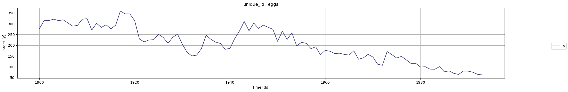
We can have a look at how the prices have evolved in the 20th century,
demonstrating that the price is trending down.
```python
nixtla_client.plot(df)
```
### Step 3: Generate Bounded Forecasts with TimeGPT
First, we transform the target data. In this case, we will log-transform the
data prior to forecasting, such that we can only forecast positive prices.
```python
df_transformed = df.copy()
df_transformed['y'] = np.log(df_transformed['y'])
```
We will create forecasts for the next 10 years, and we include an 80, 90 and
99.5 percentile of our forecast distribution.
```python
timegpt_fcst_with_transform = nixtla_client.forecast(
df=df_transformed,
h=10,
freq='Y',
level=[80, 90, 99.5]
)
```
After having created the forecasts, we need to inverse the transformation that
we applied earlier. With a log-transformation, this simply means we need to
exponentiate the forecasts:
```python
cols_to_transform = [
col for col in timegpt_fcst_with_transform if col not in ['unique_id', 'ds']
]
for col in cols_to_transform:
timegpt_fcst_with_transform[col] = np.exp(timegpt_fcst_with_transform[col])
```
Now, we can plot the forecasts. We include a number of prediction intervals,
indicating the 80, 90 and 99.5 percentile of our forecast distribution.
```python
nixtla_client.plot(
df,
timegpt_fcst_with_transform,
level=[80, 90, 99.5],
max_insample_length=20
)
```
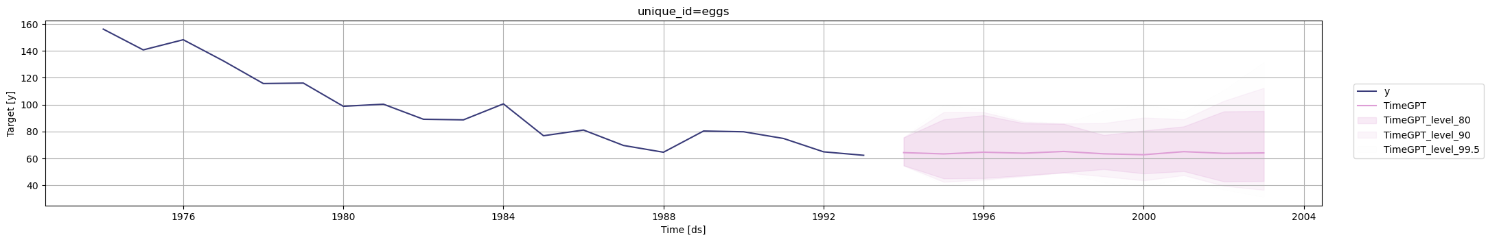
The forecast and the prediction intervals look reasonable.
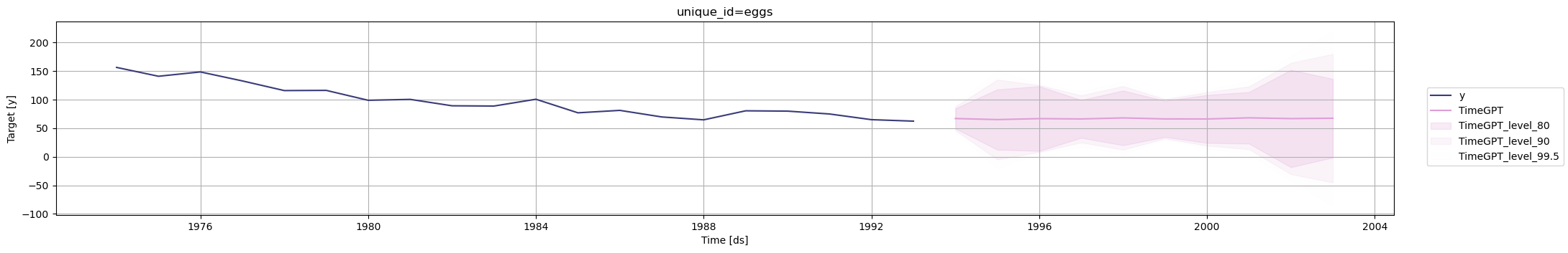
### Step 4: Compare with Unbounded Forecast
Let's compare these forecasts to the situation where we don't apply a
transformation. In this case, it may be possible to forecast a negative price.
```python
timegpt_fcst_without_transform = nixtla_client.forecast(
df=df,
h=10,
freq='Y',
level=[80, 90, 99.5]
)
```
Indeed, we now observe prediction intervals that become negative:
```python
nixtla_client.plot(
df,
timegpt_fcst_without_transform,
level=[80, 90, 99.5],
max_insample_length=20
)
```
For example, in 1995:
```python
timegpt_fcst_without_transform
```
| | unique_id | ds | TimeGPT | TimeGPT-lo-99.5 | TimeGPT-lo-90 | TimeGPT-lo-80 | TimeGPT-hi-80 | TimeGPT-hi-90 | TimeGPT-hi-99.5 |
|--:|----------:|-----------:|----------:|----------------:|--------------:|--------------:|--------------:|--------------:|----------------:|
| 0 | eggs | 1994-01-01 | 66.859756 | 43.103240 | 46.131448 | 49.319034 | 84.400479 | 87.588065 | 90.616273 |
| 1 | eggs | 1995-01-01 | 64.993477 | -20.924112 | -4.750041 | 12.275298 | 117.711656 | 134.736995 | 150.911066 |
| 2 | eggs | 1996-01-01 | 66.695808 | 6.499170 | 8.291150 | 10.177444 | 123.214173 | 125.100467 | 126.892446 |
| 3 | eggs | 1997-01-01 | 66.103325 | 17.304282 | 24.966939 | 33.032894 | 99.173756 | 107.239711 | 114.902368 |
| 4 | eggs | 1998-01-01 | 67.906517 | 4.995371 | 12.349648 | 20.090992 | 115.722042 | 123.463386 | 130.817663 |
| 5 | eggs | 1999-01-01 | 66.147575 | 29.162207 | 31.804460 | 34.585779 | 97.709372 | 100.490691 | 103.132943 |
| 6 | eggs | 2000-01-01 | 66.062637 | 14.671932 | 19.305822 | 24.183601 | 107.941673 | 112.819453 | 117.453343 |
| 7 | eggs | 2001-01-01 | 68.045769 | 3.915282 | 13.188964 | 22.950736 | 113.140802 | 122.902573 | 132.176256 |
| 8 | eggs | 2002-01-01 | 66.718903 | -42.212631 | -30.583703 | -18.342726 | 151.780531 | 164.021508 | 175.650436 |
| 9 | eggs | 2003-01-01 | 67.344078 | -86.239911 | -44.959745 | -1.506939 | 136.195095 | 179.647901 | 220.928067 |
## Conclusion
Log-transformations are a simple and effective way to enforce non-negative
predictions. This tutorial demonstrated how TimeGPT accommodates bounded
forecasts to enhance forecast realism and reliability.
## References
- [**Hyndman, Rob J., and George Athanasopoulos (2021). Forecasting: Principles and Practice (3rd Ed)**](https://otexts.com/fpp3/)