---
title: "Fine-tuning with a Specific Loss Function"
description: "Learn how to fine-tune a model using specific loss functions, configure the Nixtla client, and evaluate performance improvements."
icon: "gear"
---
## Fine-tuning with a Specific Loss Function
When you fine-tune, the model trains on your dataset to tailor predictions to
your specific dataset. You can specify the loss function to be used during
fine-tuning using the `finetune_loss` argument. Below are the available loss
functions:
* `"default"`: A proprietary function robust to outliers.
* `"mae"`: Mean Absolute Error
* `"mse"`: Mean Squared Error
* `"rmse"`: Root Mean Squared Error
* `"mape"`: Mean Absolute Percentage Error
* `"smape"`: Symmetric Mean Absolute Percentage Error
## How to Fine-tune with a Specific Loss Function
[](https://colab.research.google.com/github/Nixtla/nixtla/blob/main/nbs/docs/tutorials/07_loss_function_finetuning.ipynb)
### Step 1: Import Packages and Initialize Client
First, we import the required packages and initialize the Nixtla client.
```python
import pandas as pd
from nixtla import NixtlaClient
from utilsforecast.losses import mae, mse, rmse, mape, smape
```
```python
nixtla_client = NixtlaClient(
# defaults to os.environ.get("NIXTLA_API_KEY")
api_key='my_api_key_provided_by_nixtla'
)
```
### Step 2: Load Data
Load your data and prepare it for fine-tuning. Here, we will demonstrate using
an example dataset of air passenger counts.
```python
df = pd.read_csv('https://raw.githubusercontent.com/Nixtla/transfer-learning-time-series/main/datasets/air_passengers.csv')
df.insert(loc=0, column='unique_id', value=1)
df.head()
```
| | unique_id | timestamp | value |
| ----- | ----------- | ------------ | ------- |
| 0 | 1 | 1949-01-01 | 112 |
| 1 | 1 | 1949-02-01 | 118 |
| 2 | 1 | 1949-03-01 | 132 |
| 3 | 1 | 1949-04-01 | 129 |
| 4 | 1 | 1949-05-01 | 121 |
### Step 3: Fine-Tune the Model
Let's fine-tune the model on a dataset using the mean absolute error (MAE).
For that, we simply pass the appropriate string representing the loss function
to the `finetune_loss` parameter of the `forecast` method.
```python
timegpt_fcst_finetune_mae_df = nixtla_client.forecast(
df=df,
h=12,
finetune_steps=10,
finetune_loss='mae', # Select desired loss function
time_col='timestamp',
target_col='value',
)
```
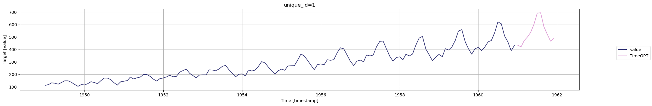
After training completes, you can visualize the forecast:
```python
nixtla_client.plot(
df,
timegpt_fcst_finetune_mae_df,
time_col='timestamp',
target_col='value',
)
```
## Explanation of Loss Functions
Now, depending on your data, you will use a specific error metric to accurately
evaluate your forecasting model's performance.
Below is a non-exhaustive guide on which metric to use depending on your use case.
**Mean absolute error (MAE)**
 = \frac{1}{H} \sum^{t+H}_{\tau=t+1} |y_{\tau} - \hat{y}_{\tau}|) - Robust to outliers
- Easy to understand
- You care equally about all error sizes
- Same units as your data
**Mean squared error (MSE)**
- Robust to outliers
- Easy to understand
- You care equally about all error sizes
- Same units as your data
**Mean squared error (MSE)**
 = \frac{1}{H} \sum^{t+H}_{\tau=t+1} (y_{\tau} - \hat{y}_{\tau})^{2}) - You want to penalize large errors more than small ones
- Sensitive to outliers
- Used when large errors must be avoided
- *Not* the same units as your data
**Root mean squared error (RMSE)**
- You want to penalize large errors more than small ones
- Sensitive to outliers
- Used when large errors must be avoided
- *Not* the same units as your data
**Root mean squared error (RMSE)**
 = \sqrt{\frac{1}{H} \sum^{t+H}_{\tau=t+1} (y_{\tau} - \hat{y}_{\tau})^{2}}) - Brings the MSE back to original units of data
- Penalizes large errors more than small ones
**Mean absolute percentage error (MAPE)**
- Brings the MSE back to original units of data
- Penalizes large errors more than small ones
**Mean absolute percentage error (MAPE)**
 = \frac{1}{H} \sum^{t+H}_{\tau=t+1} \frac{|y_{\tau}-\hat{y}_{\tau}|}{|y_{\tau}|}) - Easy to understand for non-technical stakeholders
- Expressed as a percentage
- Heavier penalty on positive errors over negative errors
- To be avoided if your data has values close to 0 or equal to 0
**Symmetric mean absolute percentage error (sMAPE)**
- Easy to understand for non-technical stakeholders
- Expressed as a percentage
- Heavier penalty on positive errors over negative errors
- To be avoided if your data has values close to 0 or equal to 0
**Symmetric mean absolute percentage error (sMAPE)**
 = \frac{1}{H} \sum^{t+H}_{\tau=t+1} \frac{|y_{\tau}-\hat{y}_{\tau}|}{|y_{\tau}|+|\hat{y}_{\tau}|}) - Fixes bias of MAPE
- Equally sensitive to over and under forecasting
- To be avoided if your data has values close to 0 or equal to 0
With TimeGPT, you can choose your loss function during fine-tuning as to
maximize the model's performance metric for your particular use case.
## Experimentation with Loss Function
Let's run a small experiment to see how each loss function improves their
associated metric when compared to the default setting.
Let's split the dataset into training and testing sets.
```python
train = df[:-36]
test = df[-36:]
```
Next, let's compute the forecasts with the various loss functions.
```python
losses = ['default', 'mae', 'mse', 'rmse', 'mape', 'smape']
test = test.copy()
for loss in losses:
preds_df = nixtla_client.forecast(
df=train,
h=36,
finetune_steps=10,
finetune_loss=loss,
time_col='timestamp',
target_col='value')
preds = preds_df['TimeGPT'].values
test.loc[:,f'TimeGPT_{loss}'] = preds
```
Great! We have predictions from TimeGPT using all the different loss functions.
We can evaluate the performance using their associated metric and measure the
improvement.
```python
loss_fct_dict = {
"mae": mae,
"mse": mse,
"rmse": rmse,
"mape": mape,
"smape": smape
}
pct_improv = []
for loss in losses[1:]:
evaluation = loss_fct_dict[f'{loss}'](test, models=['TimeGPT_default', f'TimeGPT_{loss}'], id_col='unique_id', target_col='value')
pct_diff = (evaluation['TimeGPT_default'] - evaluation[f'TimeGPT_{loss}']) / evaluation['TimeGPT_default'] * 100
pct_improv.append(round(pct_diff, 2))
```
```python
data = {
'mae': pct_improv[0].values,
'mse': pct_improv[1].values,
'rmse': pct_improv[2].values,
'mape': pct_improv[3].values,
'smape': pct_improv[4].values
}
metrics_df = pd.DataFrame(data)
metrics_df.index = ['Metric improvement (%)']
metrics_df
```
| | mae | mse | rmse | mape | smape |
| ------------------------ | ------ | ------ | ------ | ------- | ------- |
| Metric improvement (%) | 8.54 | 0.31 | 0.64 | 31.02 | 7.36 |
From the table above, we can see that using a specific loss function during
fine-tuning will improve its associated error metric when compared to the
default loss function.
In this example, using the MAE as the loss function improves the metric by
8.54% when compared to using the default loss function.
That way, depending on your use case and performance metric, you can use the
appropriate loss function to maximize the accuracy of the forecasts.
- Fixes bias of MAPE
- Equally sensitive to over and under forecasting
- To be avoided if your data has values close to 0 or equal to 0
With TimeGPT, you can choose your loss function during fine-tuning as to
maximize the model's performance metric for your particular use case.
## Experimentation with Loss Function
Let's run a small experiment to see how each loss function improves their
associated metric when compared to the default setting.
Let's split the dataset into training and testing sets.
```python
train = df[:-36]
test = df[-36:]
```
Next, let's compute the forecasts with the various loss functions.
```python
losses = ['default', 'mae', 'mse', 'rmse', 'mape', 'smape']
test = test.copy()
for loss in losses:
preds_df = nixtla_client.forecast(
df=train,
h=36,
finetune_steps=10,
finetune_loss=loss,
time_col='timestamp',
target_col='value')
preds = preds_df['TimeGPT'].values
test.loc[:,f'TimeGPT_{loss}'] = preds
```
Great! We have predictions from TimeGPT using all the different loss functions.
We can evaluate the performance using their associated metric and measure the
improvement.
```python
loss_fct_dict = {
"mae": mae,
"mse": mse,
"rmse": rmse,
"mape": mape,
"smape": smape
}
pct_improv = []
for loss in losses[1:]:
evaluation = loss_fct_dict[f'{loss}'](test, models=['TimeGPT_default', f'TimeGPT_{loss}'], id_col='unique_id', target_col='value')
pct_diff = (evaluation['TimeGPT_default'] - evaluation[f'TimeGPT_{loss}']) / evaluation['TimeGPT_default'] * 100
pct_improv.append(round(pct_diff, 2))
```
```python
data = {
'mae': pct_improv[0].values,
'mse': pct_improv[1].values,
'rmse': pct_improv[2].values,
'mape': pct_improv[3].values,
'smape': pct_improv[4].values
}
metrics_df = pd.DataFrame(data)
metrics_df.index = ['Metric improvement (%)']
metrics_df
```
| | mae | mse | rmse | mape | smape |
| ------------------------ | ------ | ------ | ------ | ------- | ------- |
| Metric improvement (%) | 8.54 | 0.31 | 0.64 | 31.02 | 7.36 |
From the table above, we can see that using a specific loss function during
fine-tuning will improve its associated error metric when compared to the
default loss function.
In this example, using the MAE as the loss function improves the metric by
8.54% when compared to using the default loss function.
That way, depending on your use case and performance metric, you can use the
appropriate loss function to maximize the accuracy of the forecasts.