---
title: "Controlling the Anomaly Detection Process"
description: "Learn how to tune TimeGPT's anomaly detection parameters for optimal accuracy. Step-by-step guide to adjusting detection_size, level, confidence intervals, and fine-tuning strategies with Python code examples."
icon: "brain"
---
## Overview
Fine-tuning anomaly detection parameters is essential for reducing false positives and improving detection accuracy in time series data. This guide shows you how to optimize TimeGPT's `detect_anomalies_online` method by adjusting key parameters like detection sensitivity, window sizes, and model fine-tuning options.
For an introduction to real-time anomaly detection, see our [Real-Time Anomaly Detection guide](/anomaly_detection/real-time/introduction). To understand local vs global detection strategies, check out [Local vs Global Anomaly Detection](/anomaly_detection/real-time/univariate_multivariate).
## Why Parameter Tuning Matters
TimeGPT leverages forecast errors to identify anomalies in your time-series data. By optimizing parameters, you can detect subtle deviations, reduce false positives, and customize results for specific use cases.
## Key Parameters for Anomaly Detection
TimeGPT's anomaly detection can be controlled through three primary parameters:
- **detection_size**: Controls the data window size for threshold calculation, determining how much historical context is used
- **level**: Sets confidence intervals for anomaly thresholds (e.g., 80%, 95%, 99%), controlling detection sensitivity
- **freq**: Aligns detection with data frequency (e.g., 'D' for daily, 'H' for hourly, 'min' for minute-level data)
## Common Use Cases
Adjusting anomaly detection parameters is crucial for:
- **Reducing false positives** in noisy time series data
- **Increasing sensitivity** to detect subtle anomalies
- **Optimizing detection** for different data frequencies (hourly, daily, weekly)
- **Improving accuracy** through model fine-tuning with custom loss functions
## How to Adjust the Anomaly Detection Process
[](https://colab.research.google.com/github/Nixtla/nixtla/blob/main/nbs/docs/capabilities/online-anomaly-detection/02_adjusting_detection_process.ipynb)
### Step 1: Install and Import Dependencies
In your environment, install and import the necessary libraries:
```python
import pandas as pd
from nixtla import NixtlaClient
import matplotlib.pyplot as plt
```
### Step 2: Initialize the Nixtla Client
Create an instance of NixtlaClient with your API key:
```python
nixtla_client = NixtlaClient(api_key='my_api_key_provided_by_nixtla')
```
### Step 3: Conduct a baseline detection
Load a portion of the Peyton Manning dataset to illustrate the default anomaly detection process. We use the Peyton Manning Wikipedia page views dataset to demonstrate parameter tuning on real-world data with natural anomalies and trends.
```python
df = pd.read_csv(
'https://datasets-nixtla.s3.amazonaws.com/peyton-manning.csv',
parse_dates=['ds']
).tail(200)
df.head()
```
| x | unique_id | ds | y |
| ------ | ----------- | ------------ | ---------- |
| 2764 | 0 | 2015-07-05 | 6.499787 |
| 2765 | 0 | 2015-07-06 | 6.859615 |
| 2766 | 0 | 2015-07-07 | 6.881411 |
| 2767 | 0 | 2015-07-08 | 6.997596 |
| 2768 | 0 | 2015-07-09 | 7.152269 |
Set a baseline by using only the default parameters of the method.
```python
anomaly_df = nixtla_client.detect_anomalies_online(
df,
freq='D',
h=14,
level=80,
detection_size=150
)
```
```bash Baseline Detection Log Output
INFO:nixtla.nixtla_client:Validating inputs...
INFO:nixtla.nixtla_client:Preprocessing dataframes...
WARNING:nixtla.nixtla_client:Detection size is large. Using the entire series to compute the anomaly threshold...
INFO:nixtla.nixtla_client:Calling Online Anomaly Detector Endpoint...
```
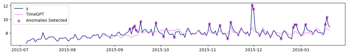
### Step 4: Fine-tuned detection
TimeGPT detects anomalies based on forecast errors. By improving your model's forecasts, you can strengthen anomaly detection performance. The following parameters can be fine-tuned:
- **finetune_steps**: Number of additional training iterations
- **finetune_depth**: Depth level for refining the model
- **finetune_loss**: Loss function used during fine-tuning
```python
anomaly_online_ft = nixtla_client.detect_anomalies_online(
df,
freq='D',
h=14,
level=80,
detection_size=150,
finetune_steps=10,
finetune_depth=2,
finetune_loss='mae'
)
```
```bash Fine-tuned Detection Log Output
INFO:nixtla.nixtla_client:Validating inputs...
INFO:nixtla.nixtla_client:Preprocessing dataframes...
WARNING:nixtla.nixtla_client:Detection size is large. Using the entire series to compute the anomaly threshold...
INFO:nixtla.nixtla_client:Calling Online Anomaly Detector Endpoint...
```

From the plot above, we can see that fewer anomalies were detected by the model, since the fine-tuning process helps TimeGPT better forecast the series.
### Step 5: Adjusting Forecast Horizon and Step Size
Similar to cross-validation, the anomaly detection method generates forecasts for historical data by splitting the time series into multiple windows. The way these windows are defined can impact the anomaly detection results. Two key parameters control this process:
* `h`: Specifies how many steps into the future the forecast is made for each window.
* `step_size`: Determines the interval between the starting points of consecutive windows.
Note that when `step_size` is smaller than `h`, then we get overlapping windows. This can make the detection process more robust, as TimeGPT will see the same time step more than once. However, this comes with a computational cost, since the same time step will be predicted more than once.
```python
anomaly_df_horizon = nixtla_client.detect_anomalies_online(
df,
time_col='ds',
target_col='y',
freq='D',
h=2,
step_size=1,
level=80,
detection_size=150
)
```

**Choosing `h` and `step_size`** depends on the nature of your data:
- Frequent or short anomalies: Use smaller `h` and `step_size`
- Smooth or longer trends: Choose larger `h` and `step_size`
## Summary
You've learned how to control TimeGPT's anomaly detection process through:
1. **Baseline detection** using default parameters
2. **Fine-tuning** with custom training iterations and loss functions
3. **Window adjustment** using forecast horizon and step size parameters
Experiment with these parameters to optimize detection for your specific use case and data patterns.
## Frequently Asked Questions
**How do I reduce false positives in anomaly detection?**
Increase the `level` parameter (e.g., from 80 to 95 or 99) to make detection stricter, or use fine-tuning parameters like `finetune_steps` to improve forecast accuracy.
**What's the difference between detection_size and step_size?**
`detection_size` determines how many data points to analyze, while `step_size` controls the interval between detection windows when using overlapping windows.
**When should I use fine-tuning for anomaly detection?**
Use fine-tuning when you have domain-specific patterns or when baseline detection produces too many false positives. Fine-tuning helps TimeGPT better understand your specific time series characteristics.
**How does overlapping windows improve detection?**
When `step_size` < `h`, TimeGPT analyzes the same time steps multiple times from different perspectives, making detection more robust but requiring more computation.