---
title: "Quickstart"
description: "Get started with TimeGPT's historical anomaly detection capabilities."
icon: "bug"
---


<CardGroup cols={2}>
  <Card title="What you'll learn" icon="circle-info">

      - Understand how TimeGPT detects anomalies in historical time series.

      - How to setup and detect anomalies with TimeGPT.

      - How to plot and interpret identified anomalies.

  </Card>
  <Card title="Key benefits" icon="circle-check">

      - Quickly identify outliers in large time series.

      - Improve decision-making by focusing on unusual data points.

      - Automate anomaly alerts to save time and resources.
  </Card>
</CardGroup>

## What Is Historical Anomaly Detection?

Historical anomaly detection is a technique that identifies data points that significantly deviate from expected patterns in a time series. This technique is useful for uncovering potential fraud, security breaches, or other unusual events.

## Overview of TimeGPT's Historical Anomaly Detection

TimeGPT's historical anomaly detection works by:

1. Generating predictions for future values (or reconstructing missing values) within your historical time series.
2. Constructing a confidence interval based on the model's predictions.
3. Flagging any historical data point that falls outside your chosen confidence interval as an anomaly.


## Quickstart Example

You'll learn how historical anomaly detection works—illustrated through an example analyzing daily visits to the Wikipedia page of Peyton Manning.

[![Open In Colab](https://colab.research.google.com/assets/colab-badge.svg)](https://colab.research.google.com/github/Nixtla/nixtla/blob/main/nbs/docs/capabilities/historical-anomaly-detection/01_quickstart.ipynb)


### Step 1: Import Packages and Create a NixtlaClient Instance

We'll start by importing required packages and setting up our API key.

```python
import pandas as pd
from nixtla import NixtlaClient

nixtla_client = NixtlaClient(
    api_key='my_api_key_provided_by_nixtla'  # Defaults to os.environ.get("NIXTLA_API_KEY")
)
```

### Step 2: Load the Dataset

This dataset tracks the daily visits to the Wikipedia page of Peyton Manning.

```python
df = pd.read_csv('https://datasets-nixtla.s3.amazonaws.com/peyton-manning.csv')
df.head()
```
|   | unique_id | ds         | y        |
|---|-----------|------------|----------|
| 0 | 0         | 2007-12-10 | 9.590761 |
| 1 | 0         | 2007-12-11 | 8.519590 |
| 2 | 0         | 2007-12-12 | 8.183677 |
| 3 | 0         | 2007-12-13 | 8.072467 |
| 4 | 0         | 2007-12-14 | 7.893572 |


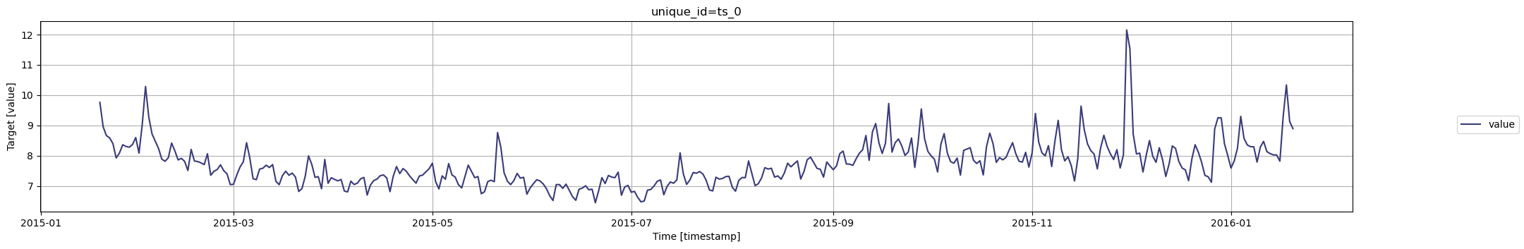
### Step 3: Visualize the Data

You can visualize the time series with the following command:

```python
nixtla_client.plot(df, max_insample_length=365)
```
    <Frame caption="Figure 1. Peyton Manning Wikipedia page visits over time." >
      ![Data plot](https://raw.githubusercontent.com/Nixtla/nixtla/readme_docs/nbs/_docs/docs/tutorials/20_anomaly_detection_files/figure-markdown_strict/cell-11-output-1.png)
    </Frame>

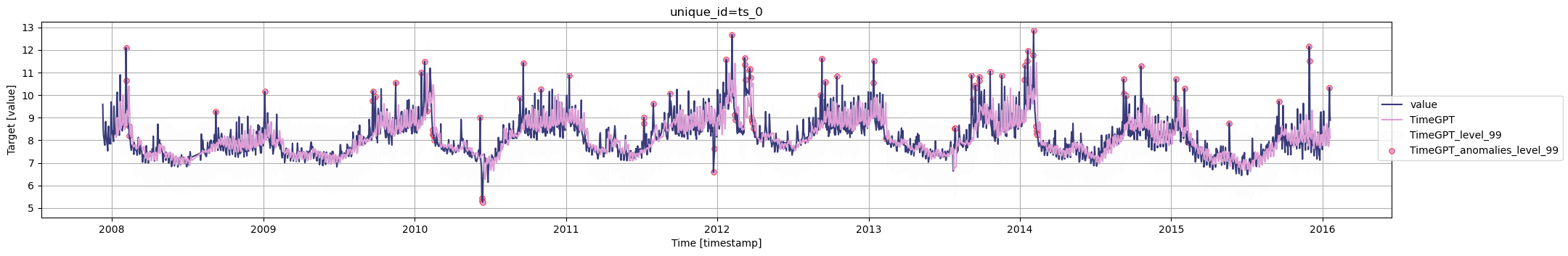
### Step 4: Perform Anomaly Detection

By default, TimeGPT uses a 99% confidence interval. Points outside this interval are flagged as anomalies.

```python
anomalies_df = nixtla_client.detect_anomalies(df, freq='D')
anomalies_df.head()
```

|   | unique_id | ds         | y        | TimeGPT  | TimeGPT-hi-99 | TimeGPT-lo-99 | anomaly |
|---|-----------|------------|----------|----------|---------------|---------------|---------|
| 0 | 0         | 2008-01-10 | 8.281724 | 8.224187 | 9.503586      | 6.944788      | False   |
| 1 | 0         | 2008-01-11 | 8.292799 | 8.151533 | 9.430932      | 6.872135      | False   |
| 2 | 0         | 2008-01-12 | 8.199189 | 8.127243 | 9.406642      | 6.847845      | False   |
| 3 | 0         | 2008-01-13 | 9.996522 | 8.917259 | 10.196658     | 7.637861      | False   |
| 4 | 0         | 2008-01-14 | 10.127071| 9.002326 | 10.281725     | 7.722928      | False   |

A `False` anomaly value indicates a normal data point; `True` identifies an outlier.

### Step 5: Review Anomalies


```python
nixtla_client.plot(df, anomalies_df)
```

<Frame caption="Figure 2. Anomalies detected in the Peyton Manning dataset.">
  ![Anomalies plot](https://raw.githubusercontent.com/Nixtla/nixtla/readme_docs/nbs/_docs/docs/tutorials/20_anomaly_detection_files/figure-markdown_strict/cell-13-output-1.png)
</Frame>

### Step 6: Inspect and Iterate

Inspect the anomalies flagged by the model. These points are potential indicators of significant deviations in your data.If you find that the model is overly sensitive or missing critical outliers, adjust the confidence interval or include additional features (e.g., exogenous data, date features) to improve detection accuracy.


<Check>
Congratulations! You've successfully performed anomaly detection using TimeGPT. You can now start experimenting with this example or apply it to your own data. For advanced tips on improving detection performance, explore the following sections on using exogenous variables and adjusting confidence intervals.
</Check>