# Fast Discounted Cumulative Sums in PyTorch
[](https://pypi.org/project/torch-discounted-cumsum/)

[](https://pepy.tech/project/torch-discounted-cumsum)
[-BSD%203--Clause-blue.svg)](LICENSE_code)
[-CC%20BY%204.0-lightgrey.svg)](LICENSE_doc)
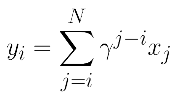 This repository implements an efficient parallel algorithm for the computation of discounted cumulative sums
and a Python package with differentiable bindings to PyTorch. The discounted `cumsum` operation is frequently seen in
data science domains concerned with time series, including Reinforcement Learning (RL).
The traditional sequential algorithm performs the computation of the output elements in a loop. For an input of size
`N`, it requires `O(N)` operations and takes `O(N)` time steps to complete.
The proposed parallel algorithm requires a total of `O(N log N)` operations, but takes only `O(log N)` time steps, which is a
considerable trade-off in many applications involving large inputs.
Features of the parallel algorithm:
- Speed logarithmic in the input size
- Better numerical precision than sequential algorithms
Features of the package:
- CPU: sequential algorithm in C++
- GPU: parallel algorithm in CUDA
- Gradients computation wrt input
- Both left and right directions of summation supported
- PyTorch bindings
## Usage
#### Installation
```shell script
pip install torch-discounted-cumsum
```
#### API
- `discounted_cumsum_right`: Computes discounted cumulative sums to the right of each position (a standard setting in RL)
- `discounted_cumsum_left`: Computes discounted cumulative sums to the left of each position
#### Example
```python
import torch
from torch_discounted_cumsum import discounted_cumsum_right
N = 8
gamma = 0.99
x = torch.ones(1, N).cuda()
y = discounted_cumsum_right(x, gamma)
print(y)
```
Output:
```
tensor([[7.7255, 6.7935, 5.8520, 4.9010, 3.9404, 2.9701, 1.9900, 1.0000]],
device='cuda:0')
```
#### Up to `K` elements
```python
import torch
from torch_discounted_cumsum import discounted_cumsum_right
N = 8
K = 2
gamma = 0.99
x = torch.ones(1, N).cuda()
y_N = discounted_cumsum_right(x, gamma)
y_K = y_N - (gamma ** K) * torch.cat((y_N[:, K:], torch.zeros(1, K).cuda()), dim=1)
print(y_K)
```
Output:
```
tensor([[1.9900, 1.9900, 1.9900, 1.9900, 1.9900, 1.9900, 1.9900, 1.0000]],
device='cuda:0')
```
## Parallel Algorithm
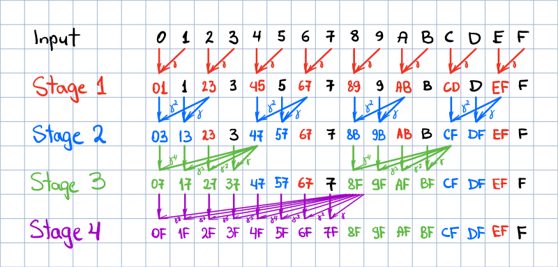
For the sake of simplicity, the algorithm is explained for `N=16`.
The processing is performed in-place in the input vector in `log2 N` stages. Each stage updates `N / 2` positions in parallel
(that is, in a single time step, provided unrestricted parallelism). A stage is characterized by the size of the group of
sequential elements being updated, which is computed as `2 ^ (stage - 1)`.
The group stride is always twice larger than the group size. The elements updated during the stage are highlighted with
the respective stage color in the figure below. Here input elements are denoted with their position id in hex, and the
elements tagged with two symbols indicate the range over which the discounted partial sum is computed upon stage completion.
Each element update includes an in-place addition of a discounted element, which follows the last
updated element in the group. The discount factor is computed as gamma raised to the power of the distance between the
updated and the discounted elements. In the figure below, this operation is denoted with tilted arrows with a greek
gamma tag. After the last stage completes, the output is written in place of the input.
This repository implements an efficient parallel algorithm for the computation of discounted cumulative sums
and a Python package with differentiable bindings to PyTorch. The discounted `cumsum` operation is frequently seen in
data science domains concerned with time series, including Reinforcement Learning (RL).
The traditional sequential algorithm performs the computation of the output elements in a loop. For an input of size
`N`, it requires `O(N)` operations and takes `O(N)` time steps to complete.
The proposed parallel algorithm requires a total of `O(N log N)` operations, but takes only `O(log N)` time steps, which is a
considerable trade-off in many applications involving large inputs.
Features of the parallel algorithm:
- Speed logarithmic in the input size
- Better numerical precision than sequential algorithms
Features of the package:
- CPU: sequential algorithm in C++
- GPU: parallel algorithm in CUDA
- Gradients computation wrt input
- Both left and right directions of summation supported
- PyTorch bindings
## Usage
#### Installation
```shell script
pip install torch-discounted-cumsum
```
#### API
- `discounted_cumsum_right`: Computes discounted cumulative sums to the right of each position (a standard setting in RL)
- `discounted_cumsum_left`: Computes discounted cumulative sums to the left of each position
#### Example
```python
import torch
from torch_discounted_cumsum import discounted_cumsum_right
N = 8
gamma = 0.99
x = torch.ones(1, N).cuda()
y = discounted_cumsum_right(x, gamma)
print(y)
```
Output:
```
tensor([[7.7255, 6.7935, 5.8520, 4.9010, 3.9404, 2.9701, 1.9900, 1.0000]],
device='cuda:0')
```
#### Up to `K` elements
```python
import torch
from torch_discounted_cumsum import discounted_cumsum_right
N = 8
K = 2
gamma = 0.99
x = torch.ones(1, N).cuda()
y_N = discounted_cumsum_right(x, gamma)
y_K = y_N - (gamma ** K) * torch.cat((y_N[:, K:], torch.zeros(1, K).cuda()), dim=1)
print(y_K)
```
Output:
```
tensor([[1.9900, 1.9900, 1.9900, 1.9900, 1.9900, 1.9900, 1.9900, 1.0000]],
device='cuda:0')
```
## Parallel Algorithm
For the sake of simplicity, the algorithm is explained for `N=16`.
The processing is performed in-place in the input vector in `log2 N` stages. Each stage updates `N / 2` positions in parallel
(that is, in a single time step, provided unrestricted parallelism). A stage is characterized by the size of the group of
sequential elements being updated, which is computed as `2 ^ (stage - 1)`.
The group stride is always twice larger than the group size. The elements updated during the stage are highlighted with
the respective stage color in the figure below. Here input elements are denoted with their position id in hex, and the
elements tagged with two symbols indicate the range over which the discounted partial sum is computed upon stage completion.
Each element update includes an in-place addition of a discounted element, which follows the last
updated element in the group. The discount factor is computed as gamma raised to the power of the distance between the
updated and the discounted elements. In the figure below, this operation is denoted with tilted arrows with a greek
gamma tag. After the last stage completes, the output is written in place of the input.
In the CUDA implementation, `N / 2` CUDA threads are allocated during each stage to update the respective elements. The
strict separation of updates into stages via separate kernel invocations guarantees stage-level synchronization and
global consistency of updates.
The gradients wrt input can be obtained from the gradients wrt output by simply taking `cumsum` operation with the
reversed direction of summation.
## Numerical Precision
The parallel algorithm produces a more numerically-stable output than the sequential algorithm using the same scalar
data type.
The comparison is performed between 3 runs with identical inputs ([code](tests/test.py#L116)). The first run casts inputs to
double precision and obtains the output reference using the sequential algorithm. Next, we run both sequential and
parallel algorithms with the same inputs cast to single precision and compare the results to the reference. The
comparison is performed using the `L_inf` norm, which is just the maximum of per-element discrepancies.
With 10000-element non-zero-centered input (such as all elements are 1.0), the errors of the algorithms are 2.8e-4
(sequential) and 9.9e-5 (parallel). With zero-centered inputs (such as standard gaussian noise), the errors are
1.8e-5 (sequential) and 1.5e-5 (parallel).
## Speed-up
We tested 3 implementations of the algorithm with the same 100000-element input ([code](tests/test.py#L154)):
1. Sequential in PyTorch on CPU (as in
[REINFORCE](https://github.com/pytorch/examples/blob/87d9a1e/reinforcement_learning/reinforce.py#L66-L68)) (Intel Xeon CPU, DGX-1)
2. Sequential in C++ on CPU (Intel Xeon CPU, DGX-1)
3. Parallel in CUDA (NVIDIA P-100, DGX-1)
The observed speed-ups are as follows:
- PyTorch to C++: 387 times
- PyTorch to CUDA: 36573 times
- C++ to CUDA: 94 times
## Ops-Space-Time Complexity
Assumptions:
- A fused operation of raising `gamma` to a power, multiplying the result by `x`, and adding `y` is counted as a
single fused operation;
- `N` is a power of two. When it isn't, the parallel algorithm's complexity is the same as with N equal to the next
power of two.
Under these assumptions, the sequential algorithm takes `N` operations and `N` time steps to complete.
The parallel algorithm takes `0.5 * N * log2 N` operations and can be completed in `log2 N` time steps
if the parallelism is unrestricted.
Both algorithms can be performed in-place; hence their space complexity is `O(1)`.
## In Other Frameworks
#### PyTorch
As of the time of writing, PyTorch does not provide discounted `cumsum` functionality via the API. PyTorch RL code
samples (e.g., [REINFORCE](https://github.com/pytorch/examples/blob/87d9a1e/reinforcement_learning/reinforce.py#L66-L68))
suggest computing returns in a loop over reward items. Since most RL algorithms do not require differentiating through
returns, many code samples resort to using SciPy function listed below.
#### TensorFlow
TensorFlow API provides `tf.scan` API, which can be supplied with an appropriate lambda function implementing the
formula above. Under the hood, however, `tf.scan` implement the traditional sequential algorithm.
#### SciPy
SciPy provides a `scipy.signal.lfilter` function for computing IIR filter response using the sequential algorithm, which
can be used for the task at hand, as suggested in this [StackOverflow](https://stackoverflow.com/a/47971187/411907)
response.
## Citation
To cite this repository, use the following BibTeX:
```
@misc{obukhov2021torchdiscountedcumsum,
author = {Anton Obukhov},
year = 2021,
title = {Fast discounted cumulative sums in PyTorch},
url = {www.github.com/toshas/torch-discounted-cumsum}
}
```